Technical User Manuals for Survey Instrument Calibration
Please login or signup to manage and calibrate your staff.
The Survey Instrumentation Calibration Technical User Manual
- 1. Introduction
- 2. EDM Baseline calibration
- 2.5 Pillar offsets survey
- 2.6 Pillar heights survey
- 6.2.1 ASCII import file format
1. Introduction
We adopted the word 'Medjil' from Whadjuk Noongar language, which means ‘accurate’ as the name for the survey instrumentation calibration portal.
The Medjil portal was developed by Landgate (the Western Australian Land Information Authority) in collaboration with the Intergovernmental Committee on Surveying and Mapping (ICSM) jurisdictions.
The portal allows the calibration of the following:
- EDM Instrumentation using standardised EDM Baselines
- EDM Baselines using standardised instruments
- Barcode staff using staff calibration range facility (refer to Staff Calibration manual for more details)
The purpose of calibrating the EDM Instrumentation (EDMI) is to establish the legal traceability of a user's instrument to the national standard of length provided by the National Measurement Institute (NMI). This is accomplished by determining the Instrument Correction and its uncertainty through a survey procedure conducted at a certified EDM Baseline. The certification of EDM Baselines are maintained by individual States and Territories.
The certification (or calibration) of EDM baselines establishes updated (or improved) distances between their pillars. The calibration of an EDMI provides distance correction specific to that instrumentation which are to be applied to measurements taken using that instrumentation (eg. EDM and prism). EDM Baselines and EDMI calibration should be conducted on a regular basis. Check your legislative requirements in your State and Territory for compliance.
The Medjil portal provides tools and reports for Levelling Staff, EDM Baseline and EDMI calibration procedures. Please refer to the specific guides that provide field calibration instructions.
This document includes reference information, encompassing mathematical equations, procedures, algorithms, and computations utilized by the Medjil portal. The calibration procedures are based on the following resources:
- “Instructions on the Verification of Electronic Distance Meters according to section 10, Weights and Measures (National Standards) Act, 1960” by Dr. J. M. Rüeger, School of Surveying, University of New South Wales
- “Instructions on the Verification of Electro-Optical Short-Range Distance Meters on Subsidiary Standards of Length in the Form of EDM Calibration Baselines", J.M.Rüeger, School of Surveying, University of New South Wales, 1984
- “Electronic Distance Measurements”, J.M.Rüeger, 1996
- Draft Verifying Authorities Handbook, 2001
- IAG resolutions at it’s XXIIth General Assembly in Birmingham, 1999
- Optics and optical instruments - Field procedures for testing geodetic and surveying instruments, ISO 17123-4:2012
- Evaluation of measurement data - Guide to the expression of uncertainty in measurement (GUM), JCGM 100:2008
- "Review of the Western Australian BASELINE Calibration Software for Electronic Distance Measuring (EDM) Instruments", prepared for the Surveyor General of New South Wales, J.M.Rüeger, 2019
- "Elementary Surveying - An Introduction to Geomatics", 14th Edition, C.D.Ghilani and P.R.Wolf, 2014
The Draft Verifying Authorities (VA) Handbook 2001 is intended for use by verifying authorities which are appointed under the provisions of Regulation 73 of the National Measurement Regulations 1999 in accordance with the National Measurement Act 1960 to verify reference standards of measurements under the provisions of Regulation 13, 30 and 31. The determination of the a priori standard deviations and the analysis of uncertainties of EDM measurements are based on the general guidelines within this handbook, ISO standards and GUM.
In this manual 'uncertainty' means 'expanded uncertainty' specified at the 95% confidenceF level. Standard deviation or standard uncertainty is specified at 68% confidence level. Users have the flexibility to adopt or modify default uncertainties and associated traceability statements as required.
2. EDM Baseline calibration
2.1 EDM Baseline designs
Since their introduction, the use of EDM Baseline has been the preferred calibration method for EDM instrumentation. There are three different EDM Baseline designs:
- Heerbrugg Design
- Aarau Design
- Hobart Design
Each EDM Baseline design aims to achieve an equal distribution of measured distances between the shortest and longest lines without any repetitions. They also allow EDMI calibration, with or without known distances (certified baseline distances), except for the Hobart design, which requires the distances to be known beforehand. Most EDM baseline designs aim to accommodate a variety of EDM instrument unit lengths. A detailed explanation of baseline design concepts is beyond the scope of this manual. For comprehensive information on baseline design, please refer to the book 'Electronic Distance Measurement' by J.M. Rüeger.
The current version of Medjil requires baseline distances to be known for all types of baselines to perform EDMI calibration. This approach is crucial for ensuring distance traceability to the national standard. Therefore, EDM Baselines must first be calibrated using NMI-certified instrument to determine the certified distances before proceeding with EDMI calibration. An additional module could potentially be developed to enable EDMI calibration without known distances. However, it is important to note that such calibrations cannot be certified under the NMI Act, and the EDMI distances obtained in this manner are not legally traceable to the national standard.
2.2 Mathematical model and observation equations for the calibration of EDM Baseline
Deriving two observation equations not only ensures that distances remain non-negative but also enhances the flexibility of the EDM Baseline survey:
Where:
Dij = Measured distance between pillars i and j (the observation)
xi = Distance from the first pillar to pillar 'i'. Distance corrected for the pillar offsets and reduced to baseline reference height
xj = Distance from the first pillar to pillar 'j'. Distance corrected for the pillar offsets and reduced to baseline reference height
zpc = Zero point correction (an additive constant of the certified EDMI)
2.3 Example: Formation of observation equations
Let's consider the following example baseline, comprising four pillars:
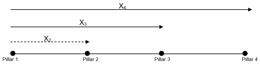
A set of linear observation equations can be formulated based on Eq. 2.1 and Eq. 2.2 as follows:
In matrix notation, the observation equations can be represented as D = AX:
Where:
Dij = Measured distance between pillars i and j (vector of the observations)
A = The design matrix
X = The certified distances and zpc (vector of the unknown output estimates)
This approach eliminates the need to provide approximate distances between pillars. In accordance with Section 6, the observations, along with their a-priori uncertainties (P), undergo a least squares adjustment to obtain the estimated certified distances dx, the zpc value, and the complete VCV matrix.
2.4 Inter-pillar distances survey
To calibrate an EDM baseline, a series of inter-pillar distance measurements (surveys) are necessary, which should include atmospheric observations of the conditions during the during measuring of each survey distance. Medjil mandates that all instrumentation used in the survey must be calibrated and possess a current certificate stating the uncertainty of the instrument readings and the calibration corrections that can be applied. The uncertainty of instrument readings plays a crucial role in propagating uncertainties for the inter-pillar distance survey.
The distance observations are assumed to be slope distances that have not been corrected for the height of instrument or height of targets. Applying atmospheric corrections by entering these into the instrument is optional but Medjil requires temperature, pressure and humidity for every distance measurement even if this has been entered into the instrument. These values are used for estimating the propagation of uncertainty as well as the optional applying of atmospheric corrections when no correction was applied by the instrument during the survey.
2.4.1 ASCII Import format
It is recommended each distance (bay) dij (where i = from_pillar; j = to_pillar) should be measured four times. However, Medjil allows the number of repeat measurements to vary between bays and between surveys.
The pillar survey data is to be provided in an ASCII file and must contain the following column headings and fields:
- from_pillar: Pillar name as defined in Medjil calibration sites
- to_pillar: Pillar name as defined in Medjil calibration sites
- height_of_instrument: Height in metres
- height_of_target: Height in metres
- horizontal_direction(dd): Angle in decimal degrees
- slope_distance: Distance in metres
- temperature: Temperature in degrees Celsius
- pressure: Pressure in Hectopascals or millibars
- humidity: Humidity in percentage
When multiple sets of meteorological instruments are specified for the pillar surveys, the additional column headings and fields are also required:
- temperature2: temperature in degrees Celsius
- pressure2: pressure in Hectopascals or millibars
- humidity2: humidity in percentage
Refer to this sample dataset required for an EDM baseline calibration survey data format.
Baseline measurements must be performed in accordance with the ISO17123-4:2012 Optics and optical instruments – Field procedures for testing geodetic and surveying instruments – Part 4: Electro-optical distance meters (EDM measurements to reflectors).
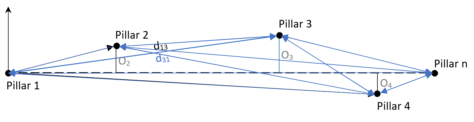
2.5 Pillar offsets survey
The pillar offset survey determines the offset of each pillar from the alignment of the first (1) and last pillar (n). Medjil performs the required reduction of observations during the EDM Baseline calibration process. Distances observed from every pillar of the baseline can be included in the calculation of the pillar offset if the survey setup includes measurements to pillar 1 and pillar n.
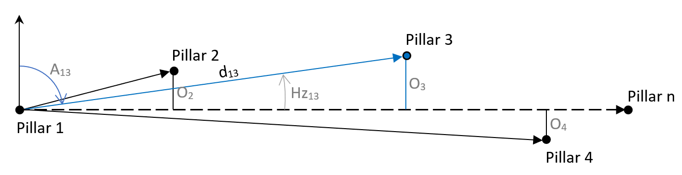
For each pillar setup, an arbitrary set of coordinates (Ej, Nj) are calculated for all pillars observed according to the formula:
Where:
dij = horizontal distance (in metres) corrected for calibration parameters and atmospheric corrections between pillars i and j
Hzij = angular direction observed at pillar i to pillar j
[Ej,Nj] = set of arbitrary coordinates (Easting and Northing) of pillar j
Then the offset of pillar j is calculated according to:
Where:
dj = horizontal distance between pillars i and j
Aj = derived bearing using coordinates of pillars: E1,N1 and Ej,Nj
As the instrument moves between pillars, pillar 1 and pillar n are observed in each setup. This allows the orientation of all setups in the survey and computation of an offset for each pillar from every pillar setup that included observations to pillar 1 and pillar n. Medjil computes the average pillar offset and standard deviation redundancy of observations measured from multiple pillars. These are used for a-priori estimation of uncertainties and the reduction of EDM measured distances to the reference alignment and height. Table 5.4 demonstrates an example set of pillar offsets.
2.6 Pillar heights survey
Pillar heights (Hj) are to be determined as orthometric heights (eg. AHD71) and provided with standard deviations. The standard deviations should preferably be derived from redundant observations. Pillar coordinates are required and used to determine the baseline location in order to derive geometric correction to the distances. Medjil uses an average latitude of the supplied pillar coordinates to calculate the geometric corrections of surveyed distances (see, Section 4.3 ).
2.6.1 ASCII Import file format
Data for the height of pillars is to be provided in an ASCII file and must contain the following column headings and fields:
- pillar_name: Pillar name as defined in Medjil calibration sites
- pillar_rl: height in metres
- rl_standard_deviation: height in metres (standard uncertainty, one sigma)
Refer to this sample dataset for the required data format.
3. EDM Instrumentation calibration
3.1 Systematic errors in EDM instruments
There are three distinct systematic errors which may occur in EDM instruments. The calibration of an instrument on a certified baseline allows to determine the specific instrument - prism correction that can eliminate of the following errors:
3.1.1 Zero Point Correction (zpc)
All distances measured by a particular EDM instrument and reflector combination (EDMI) are subject to a constant error caused by the following factors:
- Electrical delays, geometrical detours and eccentricities in the instruments
- Differences between the electronic centre and the mechanical centre of the instrument
- Differences between the optical and mechanical centres of the reflector (prism)
This errors may vary with changes of reflector, or after jolts, or with different instrument mountings. Zpc is an algebraic constant applied directly to every measurement.
3.1.2 Scale Correction Factor (scf)
Scale Correction Factor is proportional to the length of the distance measured and is caused by:
- Internal frequency errors, including those caused by external temperature and instrument “warm up” effects
- Errors of measured temperature, pressure and humidity affect the velocity (and path?) of the electromagnetic wave
- Non-homogeneous emissions/reception patterns from the emitting and receiving diodes (phase inhomogeneities)
3.1.3 Cyclic Errors
The precision of an EDM instrument dependents on the precision of the internal phase measurements. Unwanted interference through electronic/optical cross talk or multi-path effects of the transmitted signal on to the received signal causes cyclic errors. The major form of the cyclic error is sinusoidal with a wavelength equal to the unit length of the instrument. The unit length is the scale on which the EDM instrument measures the distance and is derived from the fine measuring frequency. Unit length is equal to one half of the modulation wavelength.
3.2 Mathematical model of the EDM Instrument Correction (IC)
Where:
IC = Instrument Correction
D = Distance
zpc = Zero Point Correction
scf = Scale Correction Factor (a.x)
Note: scf as (a.x) = scf - 1, where scf is expressed as (A.x)
Corrected Distance = scf * d + zpc, where scf is expressed as (A.x)
Instrument Correction = scf * d + zpc, where scf is expressed as (a.x)
Instrument Correction = scf * d * 1e-6 + zpc, where scf is expressed as scf (ppm)
U = Instrument Unit Length (m) - wavelength/2
1C, 2C, 3C and 4C = Cyclic (short periodic) parameters
By default Medjil estimates only zpc and scf. However, Medjil is also capable of solving for cyclic error parameters (1C,2C,3C,4C) which depend on wavelength cycle errors. Solving for cyclic error is optional as the ability to detect this error reliably depends on the baseline design. Aarau, Heerbrugg, and Hobart baseline designs are typically tailored for instruments with specific unit lengths. If the instrument calibration was done on a baseline not specifically designed for its unit length, or if the accuracy of cyclic errors are not suitable, the user should consider performing additional calibration on the "cyclic error" testline.
3.3 Observation equations
For every distance measured on a EDM baseline the following observation equation can be derived:
Where:
vi = Residual is the difference between certified distance and the adjusted observed distance
The angular values (sin and cos values) are expressed in radians.
Further the n observation equations for all distances measured on a certified baseline can be expressed in a matrix form as
Where:
A weight matrix can also be determined for the observed distances as:
Where:
SD = a priori standard deviation of the measured distance D
Refer to Section 4 for the derivation of the uncertainties of a measured distance. The observations together with a-priori uncertainties (p) are least squares adjusted as per Section 6. Note the weight matrix has the option to be additionally scaled by a variance factor.
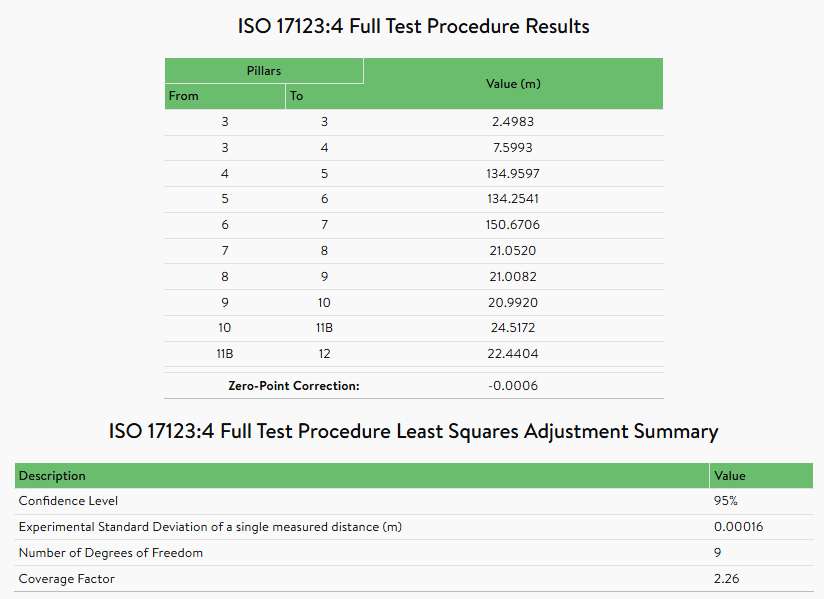
3.4 ISO full test procedure
The full test procedure is performed in accordance with ISO 17123-4:2012 and aims to determine the measure of precision (Type A evaluation of standard deviation) of a particular EDM instrumentation (EDM and its ancillary equipment) under the actual field conditions. The procedure is based on a least squares adjustment of all measured distances on an EDM Basline without known (certified) distances. The experimental standard deviation of a single distance is determined. Note this procedure cannot determine the scale factor error of the EDM instrumentation.
The ISO full test procedure results and least squares adjustment summary is provided in EDMI Calibration Report as shown in this example:
3.5 ASCII import file format
It is recommended each distance (bay) dij (where i = from_pillar; j = to_pillar) should be measured four times. However, Medjil allows the number of repeat measurements to vary between bays and between surveys.
The pillar survey data is to be provided in an ASCII file and must contain the following column headings and fields:
- from_pillar: Pillar name as defined in Medjil calibration sites
- to_pillar: Pillar name as defined in Medjil calibration sites
- height_of_instrument: Height in metres
- height_of_target: Height in metres
- slope_distance: Distance in metres
- temperature: Temperature in degrees Celsius
- pressure: Pressure in Hectopascals or millibars
- humidity: Humidity in percentage
Refer to this sample dataset for the required data format.
4. Corrections
4.1 Calibration Correction
Medjil maintains an instrument register that catalogues all instruments used for calibrations. Instrument register belongs to an individual company. The registry includes the archive of calibration certificates for EDMI, Barometer, Thermometer and Hygrometer. If calibration corrections have not been applied to instrument readings, Medjil allows calibration corrections to be applied to the raw readings during the Medjil calibration.
Data from one or two meteorological instruments (e.g. two thermometers, two barometers) can be recorded and imported to Medjil. If a set of two instruments have been used along the observed distance (e.g. at the instrument and target locations) Medjil will compute and apply averaged values.
4.1.1 Meteorological instrumentation corrections
All meteorological instruments (thermometer, barometer, hygrometer) can reference calibration certificates to apply corrections to raw readings. These corrections are sourced from the most recent instrument calibration certificate current prior to the date of pillar survey. Calibration corrections are applied as zero point correction (zpc) to the raw meteorological instruments readings:
4.1.2 EDMI correction
EDMI calibration corrections are sourced from the most recent instrument calibration certificate current prior to the date of baseline survey:
If the meteorological corrections have not been applied to EDMI readings prior to upload, atmospheric calibration corrections will be applied prior to calculating the first velocity correction.
4.2 Atmospheric correction
4.2.1 First velocity correction (K)
Where:
K = First velocity correction in metres
P = Pressure in millibars/hectopascals
t = Dry temperature in degrees Celsius
d = Distance in metres
e = Partial water pressure in hectopascals
$$C = (N_{REF} – 1)10^6$$
nREF = Reference refractive index (Section 4.2.2)
$$D = (n_G – 1) 10^6 (273.15 / 1013.25)\ \ \ \ (Eq. 4.2)$$
nG = Group refractive index of atmosphere for standard conditions
Partial vapour pressure is derived from relative humidity:
Where:
e = Partial water vapour pressure in hectopascals
h = Relative humidity in percent
E = Saturation water vapour pressure (hPa) at the dry bulb temperature:
Where:
p = Atmospheric pressure in hectopascals
t = Dry temperature in degrees Celsius
The terms C and D as well as EDM type, Unit Length, Modulation Frequency, Carrier Wavelength and Refractive Index are instrument specific (manufacturers supplied). Recommended values for common instruments are provided in the EDM Specifications Lookup Table. This table has been populated with information from the following sources:
- Rüeger, J. M. 1996. Electronic Distance Measurement - An Introduction, 4th corrected edition
- Rüeger. J. M. 2007a. First Velocity Correction in EDM: How to get the Constants C and D, Azimuth
- https://www.land.vic.gov.au/surveying/services/equipment-calibration-services
- CR Kennedy
- Topcon / Sokkia EDM Specification for Oceania Models curtesy of Aptella
- Trimble survey support bulletin - Atmospheric_Correction_Trimble TS_Ver 240_2021-02-16
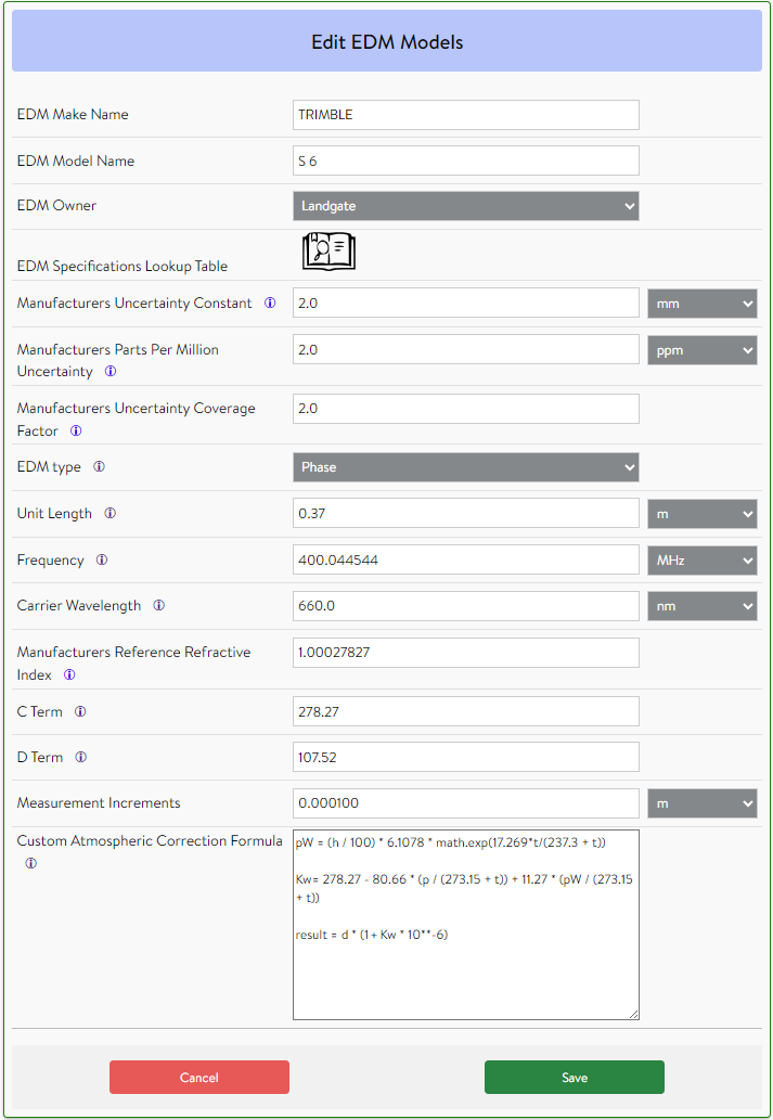
These parameters are assigned to the EDM model and are used for all instruments of that model associated with the company. The Manufacturers Uncertainty Constant, Manufacturers Parts Per Million Uncertainty and Manufacturers Uncertainty Coverage Factor are required fields. Most manufacturers state the accuracy of their instruments as a standard deviation at 68% confidence level (J.M.Rüeger, 1996). These 68% confidence level values must be multiplied by the corresponding coverage factor to determine the uncertainty. If the coverage factor is unknown, a value of 2.0 can generally be adopted. For example, if a manufacturer specifies accuracy of (1 + 1.5ppm). The values entered for Medjil instrument model specifications should be (2 + 3ppm) where k=2.0. Manufacturers Uncertainty parameters are used by Medjil to perform the statistical test recommended in ISO 17123-4:2012 (see Section 7).
Medjil treats phase and pulse measuring instruments differently (first velocity correction is different) thus pulse instruments must have mets applied before importing data to Medjil.
Solving for cyclic errors can be performed for both types of instruments and is an option when performing and EDMI Calibration.
When solving for cyclic errors, Medjil will use a t-student test for both the first and second order cyclic errors. If errors are statistically insignificant, the design matrix will be compiled for either six, four or two parameters.
The Unit Length is a required field. It is used when testing for cyclic errors, plotting the Return Phase Angle of Observed Distances plot at the end of the EDMI Calibration report, and for calculating the manufacturer's reference refractive index when it has not been supplied in this form (See Section 4.2.2).
The Frequency, Carrier Wavelength, Manufacturer's Reference Refractive Index, C Term, and D Term are optional fields. These are used for calculating the atmospheric corrections for instruments. However, Medjil will refuse to process raw data where the atmospheric corrections have not been applied prior to upload if insufficient parameters are supplied to calculate the atmospheric corrections. The C Term and D Term are used to calculate the first velocity correction (See Section 4.2.1). If the C or D Term are not supplied, Medjil uses the carrier wavelength, frequency, and manufacturer's reference refractive index to calculate these terms.
The Measurement Increments are a required field. Medjil will use this value for propagation of uncertainty when the pre-selected Uncertainty Budget requests instrument rounding to be included in the Instrument Register Record – Uncertainty Budget Sources (See Section 5.2).
The Custom Atmospheric Correction Formula is an optional field. If this field is provided, Medjil will use this formula to calculate the atmospheric corrections for EDM Instrumentation calibrations. This functionality allows instrument-specific onboard software formulas to be defined and used. If the Custom Atmospheric Correction Formula is not supplied, Medjil uses the C Term and D Term to calculate the atmospheric correction.
4.2.2 Reference Refractive Index
The reference refractive index (nREF) is instrument specific and it is preferred that the manufacturer supplied value is used rather than calculated as the rounding error of the calculated value can be significant. If the refractive index is not provided Medjil uses Unit Length, Carrier Wavelength and Modulation Frequency stored in the instrument register to calculate this value.
Where:
CO = Velocity of light in a vacuum = 299 792 458 m/s (SI definition)
λMOD = Carrier wavelength of the instrument
fMOD = Modulation frequency of the instrument
U = The half of λMOD , called the unit length of the instrument.
4.2.3 Group refractive Index of light in the atmosphere
In electro-optical EDM, the refractive index is dependent on the wavelength of the visible or infrared radiation. Different frequencies have the same propagation velocity in a vacuum, but not in air because of the interference occurrence between the different frequencies. The signal resulting from the sum of all frequencies will have the so-called group velocity, which is always smaller than the phase velocities of its individual frequencies.
Resolution 3 from the International Association of Geodesy (IAG) in 1999 at its XXIIth General Assembly in Birmingham, made the following recommendations.
- Subparagraphs (a) and (b) of Resolution No. 1 of the 13th General Assembly of IUGG (Berkeley 1963) be cancelled
- The group refractive index in air for electronic distance measurement to better than one part per million (ppm) with visible and near-infrared waves in the atmosphere be computed using the computer procedure published by Ciddor & Hill in Applied Optics (1999, Vol. 38, No. 9, 1663-1667) and Ciddor in Applied Optics (1996, Vol. 35, No. 9, 1566-1573)
- The following closed formulae be adopted for the computation of the group refractive index in air for electronic distance measurement (EDM) to within 1 ppm with visible and near-infrared waves in the atmosphere:
The following closed formulae relates to recommendation three for the computation of the group refractive index in air for electronic distance measurements:
Where:
NL = Group refractivity of visible and near infrared waves in ambient moist air. Valid for atmospheric conditions described by t, p and e
nL = Corresponding group refractive index
NG = Group refractivity index for standard conditions (visible light in dry air at 0 C, 1013.25 hPa, partial water vapour pressure = 0 and the air contains 0.0375 % CO2). See Equation 4.7.
t = Dry bulb temperature of air (C).
p = Atmospheric pressure in hectopascals
e = Partial water vapour pressure (hPa)
Where:
λ = carrier wavelength in micrometres (μm) in a vacuum These closed formulae (Eq. 4.6 and 4.7) deviate less than 0.25 ppm from the accurate formulae between -30 C and +45 C, at 1000 hPa pressure, 100% relative humidity (without condensation) and for wavelengths between 650 nm and 850 nm. The 1.0 ppm stated in recommendation 3 of resolution 3 makes some allowance for anomalous refractivity and the uncertainty in the determination of the atmospheric parameters.
Recommendation 2 and 3 have been applied in the Medjil software where atmospheric corrections have not been applied to the uploaded EDM observation data. The formulae for recommendation 2 are used for calibrating a baseline. The formulae for recommendation 3 are used for calibrating EDM Instrumentation.
4.3 Geometric Corrections
All certified distances on a calibrated baseline are on the same horizontal plane at a specified reference height and on the same vertical plane running through the first and last pillars.
The geometric corrections contain four components:
- Horizontal offset correction
- Slope correction
- Correction to the specified reference height of the baseline
- Chord-to-Arc correction
Pillar coordinates and elevation are required and used to determine the baseline location to derive geometric correction of the distances. Medjil computes an average value of the supplied coordinates.
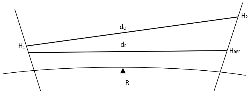
Where:
dR = Certified horizontal distance between two pillars reduced to a reference elevation HREF
H1 = Elevation of EDM instrument pillar + HEDM
H2 = Elevation of reflector pillar + HREF
HEDM = Height of EDM instrument above pillar
HREF = Height of reflector above pillar
dO= Mean observed distance between EDM instrument and reflector as corrected for atmospheric effects
ΔH = H1 – H2
HREF = Reference Elevation
O1 =Offset at pillar 1 from the straight line between the first and last pillars
O2 = Offset at pillar 2 from the straight line between the first and last pillars
R =Mean radius of curvature of the Earth at the baseline location.
To convert a certified horizontal distance between two pillars to a slope distance between the tops of these pillars the following equations is used:
Where:
dR = Certified horizontal distance between two pillars reduced to a reference elevation HREF
dX = Slope distance between the tops of two pillars
H1 = Elevation of EDM instrument pillar + HEDM
H2 = Elevation of reflector pillar + HREF
HEDM = Height of EDM instrument above pillar
HREF = Height of reflector above pillar
dO= Mean observed distance between EDM instrument and reflector as corrected for atmospheric effects
ΔH = H1 – H2
HREF = Reference Elevation
O1 = Offset at pillar 1 from the straight line between the first and last pillars
O2 = Offset at pillar 2 from the straight line between the first and last pillars
R = Mean radius of curvature of the Earth at the baseline location.
The geometric correction equations 4.8 and 4.9 were derived from The Australian Geodetic Datum Technical Manual, National Mapping Council of Australia, Special Publication 10 and are suitable for baselines with steep gradients.
Medjil uses the GRS80 spheroid for determining the mean radius of the earth (R) used in the calculation of the geometric correction. Medjil requires UTM coordinates to be specified for all EDMI calibration pillars. These coordinates are used along with the following formula to determine R for each geometric correction (GDA2020 technical manual pp. 47).
Where:
p = Radius of curvature of the spheroid in meridian
v = Radius of curvature of the spheroid in prime vertical
a = Semi-major axis of the spheroid
f = Flattening of the spheroid
Q = Latitude of the baseline location
5. Uncertainties
Medjil uses the following terminology:
- ‘Uncertainty’ refers to the GUM’s ‘expanded uncertainty' (95% confidence level or two sigmas)
- ‘Standard deviation’ refers to the GUM’s ‘standard uncertainty’ (68% confidence level or one sigma)
- ‘Coverage factor’ numerical factor used as a multiplier of the standard uncertainty in order to obtain an expanded uncertainty
Medjil adheres to the recommendation outlined in ISO 17123-4:2012, Section 6.5. It allows the definition of an uncertainty budget by combining individual sources of uncertainty (Type A and Type B) to derive combined standard uncertainty and expanded uncertainty as a representative measure of accuracy.
5.1 Combined standard and expanded uncertainty
The combined standard uncertainty CSU of a number of individual uncertainty sources (ui) is computed using the following formula:
The combined expanded uncertainty CEU is defined as follows:
Where:
k = coverage factor
veff = effective degrees of freedom
Where:
vi = degrees of freedom of an uncertainty source (i)
t = t-student distribution (probability, effective degrees of freedom)
5.2 Uncertainty budget
An uncertainty budget consists of a table of uncertainty sources that contribute to the combined uncertainty. Medjil provides a default uncertainty budget but also permits the creation of 'Custom' (company-specific) uncertainty budgets that can be select during the calibration process.
The uncertainty budget is composed of the following types of uncertainty budget sources:
- Instrument Register Record - Uncertainty Budget Sources The values for these uncertianties are sourced from values in the instrument register and may relate to the instrument parameters or the calibration certificates.
- Derived - Uncertainty Budget Sources The values for these uncertainties are derived during the computations.
- Custom - Uncertainty Budget Sources These uncertainties are entered directly. The method used to propagate this uncertainty will be according to the assigned group.
5.2.1 Custom uncertainty budgets
The Medjil ‘Default’ uncertainty budget has all options in the 'Instrument Register Record - Uncertainty Budget Sources' and 'Derived - Uncertainty Budget Sources' selected. It also defines six 'Custom - Uncertainty Budget Sources' that are appropriate for typical calibrations.
When creating a Custom uncertainty budget, Medjil will use the Default as a template to initiate the creation of the new uncertainty budget.

Where:
Name = Custom uncertainty budget name. Uncertainty budgets are identified by a name that must be unique.
Company = The owner of the new uncertainty budget. The new budget(s) are accessible to any user within that company.
Std Dev Used When Statistically Zero = This value is used to overruled (overwrite) any standard deviation equal to zero. For example Medjil uses the sample standard deviation of observation sets composed of measurements between the same pillars to calculate an uncertainty of the EDMI measurements. When all measurements in the one observation set are the same or if there is only one measurement in the observation set, the sample standard deviation is mathematically zero.
Type = Definition of uncertainty type. Type A means a statistically derived component or uncertainty where Type B stands for any other derivation of uncertainty e.g. calibration report, manufacturer's specification or an estimate based on experience.
Distribution = Definition of distribution associated with the uncertainty. A normal distribution is most associated with continuous univariate distributions such as many random variables. A rectangular distribution represents an arbitrary outcome that lies between certain bound (equal probability anywhere within the range). For example rounding of a physical quantity or a resolution of digital instrument.
Uncertainty = The expanded uncertainty at 95% confidence in the units specified for the uncertainty source.
K = The coverage factor is used to expand the uncertainty from 68% confidence level to 95% confidence level. Typically k=2.0 for a normal distribution or sqrt(3) for a rectangular distribution. Medjil will auto complete this field as the distribution drop-down is changed but the user still has the ability to overwrite this field.
Dof = Degrees of freedom. For a Type A uncertainty this is equal to the number of measurements minus the number of unknowns (redundant measurements). For a Type B uncertainty Dof needs to be estimated. The following can be used as a guide: 3 for not very confident, 10 for moderate confidence, 30 for very confident.
Group = Uncertainty sources are categorised into 11 different groups. The group selected for an uncertainty source will affect the following:
- The combining of error sources in the calibration report
- The unit selection for this uncertainty source
- The propagation (contribution) of the error sources to the total uncertainty of the calibration
EDM scale factor = Uncertainty related to the EDM scale factor can be specified in parts per million (ppm), percent (%) or scalar(a.x). All error sources belonging to this group will be combined before the contribution to the total uncertainty of the calibration according to the following formula:
Where:
sud = Standard uncertainty of the distance
D = Distance
csug = Combined standard uncertainty of the group
The 'Default' Uncertainty Budget lists an error source with the description 'EDM scale factor affected by Temp (Type B)'. The EDM scale factor can be affected by temperature. This uncertainty component is a Type B estimate based on prior knowledge and experience.
EDMI measurement = Uncertainty relating to the EDMI measurement can be specified in metres (m), millimetres (mm), parts per million (ppm), percent (%) or scalar(a.x). All error sources belonging to this group will be combined before the contribution to the total uncertainty of the calibration according to the following formula:
Where:
sud = Standard uncertainty of the distance
csug = Combined standard uncertainty of the group
EDM LS zero offset = Uncertainty relating to the EDM Least Squares zero offset can be specified in metres (m) or millimetres (mm). All error sources belonging to this group will be combined before the contribution to the total uncertainty of the calibration according to the following formula 5.7
Temperature = Uncertainty related to the temperature can be specified in degrees Celsius (°C) or degrees Fahrenheit (°F). All error sources belonging to this group will be combined before the contribution to the total uncertainty of the calibration according to the following formula:
Where:
sud = Standard uncertainty of the distance
D = Distance
csug = Combined standard uncertainty of the group
K = Partial differential for temperature defined as:
Where:
p = Pressure [hPa]
t = Temperature [C]
nG = Manufacturers reference refractive index
e = Partial water vapour Pressure [hPa] defined as:
Where:
E = Saturation water vapour [hPa] at the dry bulb temperature
h = Relative humidity [%]
Pressure = Uncertainty related to the pressure can be specified in millibars (mBar), hectopascals (hPa) or millimetres of mercury (mmHg). All error sources belonging to this group will be combined before the contribution to the total uncertainty of the calibration according to the following formula:
Where:
sud = Standard uncertainty of the distance
D = Distance
csug = Combined standard uncertainty of the group
L = Partial differential for Pressure defined as:
Humidity = Uncertainty relating to the humidity must be specified as a percent (%). All error sources belonging to this group will be combined before the contribution to the total uncertainty of the calibration according to the following formula:
Where:
sud = Standard uncertainty of the distance
D = Distance
csug = Combined standard uncertainty of the group
M = Partial differential for humidity defined as:
Certified distances = Uncertainty relating to the certified distances can be specified in metres (m), millimetres (mm), parts per million (ppm), percent (%) or scalar(a.x). All error sources belonging to this group will be combined before the contribution to the total uncertainty of the calibration according to the following formula:
Where:
sud = Standard uncertainty of the distance
csug = Combined standard uncertainty of the group
EDMI calibration = Uncertainty relating to the EDMI calibration can be specified in metres (m) or millimetres (mm). All error sources belonging to this group will be combined before the contribution to the total uncertainty of the calibration according to the Eq. 5.15.
Centring = Uncertainty relating to the centring can be specified in metres (m) or millimetres (mm). All error sources belonging to this group will be combined before the contribution to the total uncertainty of the calibration according to the Eq. 5.15.
Heights = Uncertainty relating to the heights can be specified in metres (m) or millimetres (mm). All error sources belonging to this group will be combined before the contribution to the total uncertainty of the calibration according to the following formula:
Where:
sud = Standard uncertainty of the distance
D = Distance
csug = Combined standard uncertainty of the group
∆H = Height difference between the from and to pillars
Offsets = Uncertainty relating to the offsets can be specified in metres (m) or millimetres (mm). All error sources belonging to this group will be combined before the contribution to the total uncertainty of the calibration according to the following formula:
Where:
sud = Standard uncertainty of the distance
D = Distance
csug = Combined standard uncertainty of the group
∆O = Difference in offset between from and to pillars
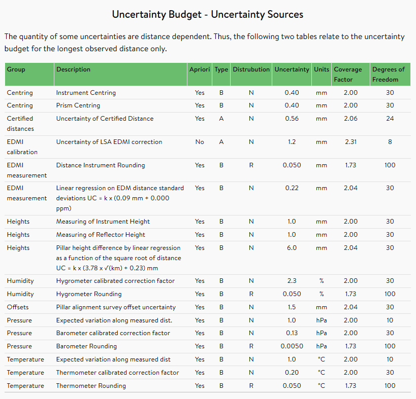
5.2.2 Uncertainty sources in reports
If the 'Default' uncertianty budget is used, Medjil automatically populates uncertainty sources shown in Table 5.1 and Table 5.2 when processing the calibration of EDM Baselines and EDM Instrumentation respectively. Except for the following, these uncertainty sources are optional when using a custom uncertainty budget:
- EDMI Calibration - Uncertainty of LSA EDMI correction
- EDM LS zero offset - ZPC uncertainty
- Certified Distances - LSA uncertainty
Table 5.1: Medjil uncertainty budget for calibration of EDM Baseline
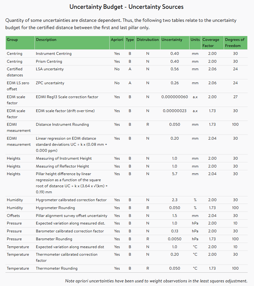
Table 5.2: Medjil uncertainty budget for calibration of EDM Instrumentation
The automatically populated uncertainty sources are defined as follows:
- Certified distances - Least Squares Adjustment (LSA) uncertainty - The uncertainty of each inter-pillar distance is uniquely assigned from the diagonal elements of the CoFactorMatrix derived from the least squares adjustment of the baseline calibration. The degrees of freedom is equal to the degrees of freedom of the calibration of the baseline and the coverage factor is derived from t-student distribution at 95% and selected degrees of freedom t(95%,dof)
- EDM LS zero offset - Zero Point Correction (ZPC) uncertainty - The uncertainty of the zero point correction is assigned from last element of the vCoFactorMatrix derived from the least squares adjustment of the baseline calibration. The degrees of freedom is equal to the degrees of freedom of the calibration of the baseline and the coverage factor is the t-student at 95% and selected degrees of freedom (t(95%,dof))
- EDM scale factor - EDMI Reg13 Scale correction factor - The uncertainty, degrees of freedom and coverage factor is assigned from the values specified in the register of calibration certificates of EDM instrument (EDMI). The selected values correspond to the most current certificate (at the time of survey) of the EDMI used for the calibration of the EDM Baseline
- EDM scale factor - EDM scale factor (drift over time) - The uncertainty is derived using linear regression of the scale factors from all available calibration certificates of the same EDM Baseline (certified distances). The scale factor is extrapolated at the time of calibration survey and the difference between this value and the last computed value (as per the most current certificate) is adopted as the uncertainty. This uncertainty source is assigned 30 degrees of freedom and a coverage factor of √3
- EDMI measurement - Distance Instrument Rounding - The uncertainty is equivalent to half of the instrument measurement increment reading. This uncertainty source is assigned 100 degrees of freedom and a coverage factor of √3.
- EDMI measurement - Linear regression on EDM distance standard deviations - Table 5.3 shows an
example of a typical subset of EDMI measurements observed on a EDM Baseline. Measurements with
the same ‘From’ and ‘To’ pillar are grouped into sets, then average and standard deviations of these
sets are tabulated. The ‘Std Dev Used when statistically zero’ field value defined in the
specified
Uncertainty Budget of the calibration can be used to exclude and overwrite experimental standard
deviations of measurement sets that have all the same values (eg. experimental standard
deviations equal to zero).
Linear regression is used on the average ‘slope distance’ and ‘standard deviation’ to derive a formula for the experimental standard deviation of EDMI measurements in the calibration: sB = P mm + Q ppm. Where sB is the standard deviation of a baseline interval.
Uncertainties are uniquely assigned to each measurement set as calculated from the derived linear regression equation. This uncertainty source is assigned 30 degrees of freedom and the coverage factor is the t-student at 95% and 30 degrees of freedom t(95%,30) - During the EDM Baseline calibration process, a *.csv file is required to upload each pillar height
and its standard deviation (standard uncertainty). These standard deviations are used to model the
standard uncertainty of each pillar height difference by linear regression as a function of the square root
of the distance. The derived line-of-best-fit equation is then used to estimate the expanded uncertainties
of height differences between pillars as a function of the square root of the distance between them (Equation 5.18).
$$ {uc}_{\Delta H_{ij}}=k*({A* \sqrt{D}+B})\ \ \ (Eq. 5.18) $$
Where:
ucΔHij = Expanded uncertainty of the height difference between pillar i and pillar j
Dij = Distance between pillar i and pillar j
A and B = parameters of the linear equation
k = t(95%,30)
- Humidity - Hygrometer calibrated correction factor - Hygrometers used for baseline calibration surveys must have a calibration certificate that indicates the uncertainty of the readings. Medjil will automatically assign a current hygrometer calibration based on the survey date. The uncertainty, coverage factor and degrees of freedom specified for that hygrometer calibration record will be used for the uncertainty ‘Humidity - Hygrometer calibrated correction factor’
- Humidity - Hygrometer rounding - The uncertainty is equivalent to half the measurement increment reading of the instrument used for the calibration. This uncertainty source is assigned 100 degrees of freedom and a coverage factor of √3.
- Offsets - Offsets - Table 5.4 shows the results of a typical alignment survey. The offset of each pillar is surveyed from multiple pillars. The offset results with the same ‘To Pillar’ are grouped into sets, then the average and experimental standard deviations of these sets are computed. When determining the uncertainty of offsets between pillars i and j, the smallest non-zero uncertainty is adopted as the combined uncertainty.
- Pressure - Barometer calibrated correction factor - Barometers used for calibration surveys must have a calibration certificate that indicates the uncertainty of the readings. Medjil will automatically assign a current barometer calibration based on the survey date. The uncertainty, coverage factor and degrees of freedom specified for that hygrometer calibration will be used for the uncertainty ‘Pressure - Barometer calibrated correction factor’
- Pressure - Barometer rounding - The uncertainty is equivalent to half the measurement increment reading of the instrument used for the calibration. This uncertainty source is assigned 100 degrees of freedom and a coverage factor of √3.
- Temperature - Thermometer calibrated correction factor - Thermometers used for calibration surveys must have a calibration that indicates the uncertainty of the readings. Medjil will automatically assign a current thermometer calibration based on the survey date. The uncertainty, coverage factor and degrees of freedom specified for that hygrometer calibration will be used for the uncertainty ‘Temperature - Thermometer calibrated correction factor’
- Temperature - Thermometer Rounding - The uncertainty is equivalent to half the measurement increment reading of the instrument used for the calibration. This uncertainty source is assigned 100 degrees of freedom and a coverage factor of √3.
- Certified distances - Uncertainty of Certified Distances - The standard uncertainty of all
inter-pillar distances are calculated from the CoFactorMatrix of baseline calibrations. This is
done by creating a design matrix for every combination of pillars and calculating another
CoFactorMatrix according to the formula:
$$ Q_2=A_2QA_2^T\ \ \ (Eq. 5.19)$$
Where:
Q2 = The secondary CoFactorMatrix
Q = The CoFactorMatrix from the LSA of calibrating a baseline
A2 = A design matrix for every possible combination of from and to pillars
The standard uncertainties of all inter-pillar distances are equivalent to the square root of the diagonals of the secondary CoFactorMatrix. These values are stored for each baseline calibration. The inter-pillar distance standard uncertainties that correspond to EDMI calibrations are used to calculate the ‘Uncertainty of Certified Distances’ according to the formula:
$$ uc_{ij} = k * S_{ij}\ \ \ (Eq. 5.20)$$Where:
ucij = Expanded uncertainty of a distance between pillar i and pillar j
k = Coverage factor of a baseline calibration determined by the t-student at 95% and LSA derived degree of freedom (dof) t(95%,dof)
Sij = Standard uncertainty of a distance between pillar i and pillar j
-
EDM Calibration - Uncertainty of LSA EDMI Correction - This is a type A uncertainty output by
the least squares adjustment used to determine calibration parameters for the calibration of EDM
Instrumentation. The uncertainty of the parameters are equivalent to the diagonal elements of
the CoFactorMatrix. The ‘Uncertainty of (LSA) EDMI Correction’ is calculated according to the
following conditions:
(a) if the calibration of the EDMI has tested for cyclic errors and found them to be significant:
$$ S_{IC}=S_{zpc}+S_{scf}D+S_1\sin{\left(2\pi\frac{D}{U}\right)+S_2\cos{\left(2\pi\frac{D}{U}\right)+S_3\sin{\left(4\pi\frac{D}{U}\right)+S_4\cos{\left(4\pi\frac{D}{U}\right)}}}}\ \ \ (Eq. 5.21)$$Where:
SIC = Standard uncertainty of the Instrument Correction
D = Distance
Szpc = Standard uncertainty of the Zero Point Correction (m)
Sscf = Standard uncertainty of the Scale Correction Factor (a.x)
U = Instrument Unit Length (m)
S1 = Standard uncertainty of the term 1 - Cyclic (a.x)
S2 = Standard uncertainty of the term 2 - Cyclic (a.x)
S3 = Standard uncertainty of the term 3 - Cyclic (a.x)
S4 = Standard uncertainty of the term 4 - Cyclic (a.x)
(b) if the calibration of the EDMI has not tested for cyclic errors, has found them to be insignificant:
$$ S_{IC}=S_{zpc}+S_{scf}D\ \ \ (Eq. 5.22)$$The uncertainty is calculated according to the following formula:
$$ {uc}_{IC}=k * S_{IC}\ \ \ (Eq. 5.23) $$Where:
uIC = Expanded uncertainty of the Instrument Correction
k = Coverage factor determined by the t-student at 95% and LSA derived degree of freedom (dof) t(95%,dof)
Table 5.3 An example set of EDMI measurements observed on a EDM Baseline
| Pillars | Raw Distances (m) | Average Distance | ||||||
|---|---|---|---|---|---|---|---|---|
| From | To | Slope Dist. 1 | Slope Dist. 2 | Slope Dist. 3 | Slope Dist. 4 | Slope Dist. 5 | Slope Dist. (m) | Dist. Std (mm) |
| 1 | 2 | 20.4005 | 20.4005 | 20.4006 | 20.4004 | 20.40050 | 0.07 | |
| 1 | 3 | 122.3877 | 122.3875 | 122.3875 | 122.3876 | 122.38758 | 0.08 | |
| 1 | 4 | 305.9899 | 305.9899 | 305.9900 | 305.9900 | 305.98995 | 0.05 | |
| 1 | 5 | 448.7901 | 448.7901 | 448.7901 | 448.7902 | 448.79013 | 0.04 | |
| 1 | 6 | 509.9729 | 509.9728 | 509.9728 | 509.9729 | 509.97285 | 0.05 | |
| 2 | 1 | 20.4009 | 20.4011 | 20.4009 | 20.4009 | 20.40095 | 0.09 | |
| 2 | 3 | 101.9871 | 101.9870 | 101.9869 | 101.9870 | 101.98700 | 0.07 | |
| 2 | 4 | 285.5891 | 285.5891 | 285.5888 | 285.5889 | 285.58898 | 0.13 | |
| 2 | 5 | 428.3894 | 428.3892 | 428.3893 | 428.3892 | 428.38928 | 0.08 | |
| 2 | 6 | 489.5733 | 489.5730 | 489.5732 | 489.5733 | 489.5730 | 489.57316 | 0.14 |
| 3 | 1 | 122.3877 | 122.3877 | 122.3877 | 122.3878 | 122.38772 | 0.04 | |
| 3 | 2 | 101.9872 | 101.9870 | 101.9870 | 101.9870 | 101.98705 | 0.09 | |
| 3 | 4 | 183.6028 | 183.6027 | 183.6027 | 183.6027 | 183.60273 | 0.04 | |
| 3 | 5 | 326.4033 | 326.4034 | 326.4034 | 326.4034 | 326.40338 | 0.04 | |
| 3 | 6 | 387.5854 | 387.5858 | 387.5856 | 387.5854 | 387.5855 | 387.58554 | 0.15 |
| 4 | 1 | 305.9901 | 305.9902 | 305.9902 | 305.9903 | 305.99020 | 0.07 | |
| 4 | 2 | 285.5894 | 285.5894 | 285.5897 | 285.5895 | 285.5896 | 285.58952 | 0.12 |
| 4 | 3 | 183.6025 | 183.6027 | 183.6026 | 183.6028 | 183.6028 | 183.60268 | 0.12 |
| 4 | 5 | 142.8025 | 142.8026 | 142.8024 | 142.8024 | 142.80248 | 0.08 | |
| 4 | 6 | 203.9846 | 203.9846 | 203.9845 | 203.9846 | 203.98458 | 0.04 | |
| 5 | 1 | 448.7904 | 448.7904 | 448.7904 | 448.7904 | 448.79040 | 0.00 | |
| 5 | 2 | 428.3904 | 428.3903 | 428.3903 | 428.3904 | 428.39035 | 0.05 | |
| 5 | 3 | 326.4035 | 326.4035 | 326.4035 | 326.4034 | 326.40348 | 0.04 | |
| 5 | 4 | 142.8027 | 142.8027 | 142.8027 | 142.8028 | 142.80272 | 0.04 | |
| 5 | 6 | 61.1820 | 61.1819 | 61.1822 | 61.1824 | 61.1823 | 61.18216 | 0.19 |
| 6 | 1 | 509.9726 | 509.9727 | 509.9728 | 509.9727 | 509.97270 | 0.07 | |
| 6 | 2 | 489.5721 | 489.5720 | 489.5722 | 489.5724 | 489.5720 | 489.57214 | 0.15 |
| 6 | 3 | 387.5860 | 387.5863 | 387.5865 | 387.5862 | 387.5862 | 387.58624 | 0.16 |
| 6 | 4 | 203.9853 | 203.9851 | 203.9852 | 203.9851 | 203.98518 | 0.08 | |
| 6 | 5 | 61.1825 | 61.1827 | 61.1827 | 61.1827 | 61.18265 | 0.09 | |
Table 5.4 An example set of alignment survey
| Surveyed From Pillar | To Pillar | Offset (m) | Average (m) | Standard Deviation (m) |
|---|---|---|---|---|
|
2
3 4 5 6 1 |
1 |
0.000
0.000 0.000 0.000 0.000 0.000 |
0.000 | 0.001 |
|
1
3 4 5 6 2 |
2 |
0.112
0.112 0.111 0.113 0.113 0.112 |
0.112 | 0.001 |
|
1
2 4 5 6 3 |
3 |
0.116
0.117 0.117 0.116 0.117 0.116 |
0.116 | 0.000 |
|
1
2 3 5 6 4 |
4 |
0.132
0.131 0.131 0.131 0.132 0.132 |
0.131 | 0.001 |
|
1
2 3 4 6 5 |
5 |
0.151
0.150 0.150 0.151 0.150 0.150 |
0.150 | 0.001 |
|
1
2 3 4 5 6 |
6 |
0.000
0.000 0.000 0.000 0.000 0.000 |
0.000 | 0.001 |
6. Least squares adjustment
6.1 Matrix notation
Residuals:
Where:
A = The design matrix
x = The vector of observations
y = The vector of the unknown output estimates
r = The vector of residuals
The least square adjustment solution:
Where:
P = The weight matrix
6.2 Detecting gross errors
Medjil performs simple detection of gross errors (outlier detection) using standardized residuals (rs):
Where:
r = The vector of residuals
σr = The vector of standard deviations of residuals
If the value of standardized residual (rs) exceeds the set rejection criteria for outlier detection (by default, two standard deviations), the observation is flagged on the graph and can be rejected form the adjustment.
6.3 Variance factor test
The Chi-square test on the variance factor is performed as a reliable statistical test to determine if the observations have been correctly weighted assuming that there are no gross errors in the observations.
Where:
σ0 is the ideal variance factor assumed to be 1.000
d is the degrees of freedom
α is the significance level of statistical testing (eg. 0.05 = 95% confidence level)
χ2 is the Chi-square distribution value
S2 is the A-posteriori variance factor
Note: Detailed description of the least squares adjustment method is out of scope of this manual. This method is widely used in surveying, geodesy and photogrammetry to solve overdetermined systems of equations based on the principle of minimising the sum of observation's residuals squares. User can explore this method in numerous available publications eg. "Practical Least Squares Adjustment of Surveying Measurements” by Alan R. Dragoo or “Adjustment Computations” by Charles D. Ghilani.
7. Calibration reports
7.1 Statistical tests
Table 7.1 provides a lists of the ISO 17123-4:2012 recommended hypothesis testing to help with the interpretation of the calibration results.
Table 7.1 List of hypothesis tests
| Test | Null hypothesis | Alternative hypothesis |
|---|---|---|
| A | s ≤ σ | s > σ |
| B | s = ε̃ | s ≠ ε̃ |
| C | δ = σ | δ ≠ σ |
The following tests assume a confidence level of 1 − α = 0.95 (95%) and a number of degrees of freedom (ν) based on number of redundant measurements.
7.1.1 Hypothesis A
This null hypothesis states that the calculated experimental standard deviation, sD, is smaller than or equal to the manufacturers specifications value σ.
The null hypothesis is not rejected if the following condition is fulfilled:
Otherwise, the null hypothesis is rejected.
The experimental standard deviations are calculated and the tests are performed for several typical distances in meters: 50, 150, 300, MaxDistance, 2xMaxDistance, 3xMaxDistance, 4xMaxDistance where the MaxDistance is the maximum distance at which the instrument was calibrated.
For detailed of calculating experimental standard deviations refer to ISO 17123:4 equation 29, Rueger (1984) equation 27 and Ghilani and Wolf (2014) equation 16.10 & Example 16.6 (4).
7.1.2 Hypothesis B
The null hypothesis states that the experimental standard deviation, s belong to the same population as the standard deviation (ε̃) obtained in the previous calibrations using the same instrumentation.
The null hypothesis is not rejected if the following condition is fulfilled:
Otherwise, the null hypothesis is rejected.
7.1.3 Hypothesis C
The null hypothesis states that the zero-point correction, δ, is equal to zero as supplied by the manufacturer (δ = 0)? Or, if prisms with a given zero-point correction, δ0 are used, is δ = δ0?
The null hypothesis is not rejected if the following condition is fulfilled:
Otherwise, the null hypothesis is rejected.
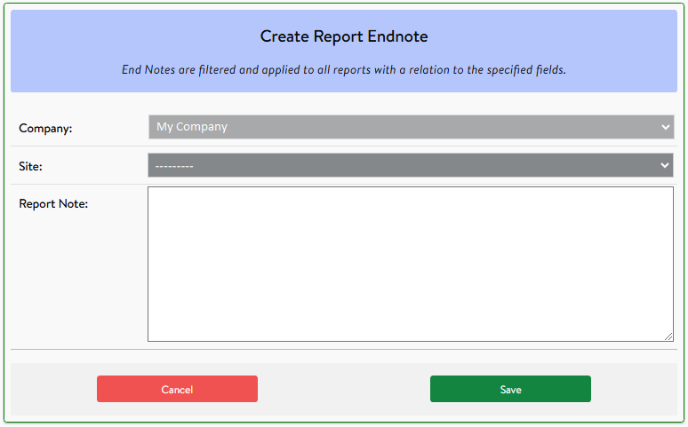
7.2 Endnotes
The EDMI and Baseline calibration reports display endnotes. These endnotes explain assumptions and decisions made during the computation of the calibration. Custom endnotes can also be predefined and applied to reports that meet the specified criteria.
7.2.1 General Users
General users are only able to apply additional endnotes to reports associated with their company. Leaving the Site: field blank will apply the endnote to all company reports. Selecting a specific Site: from the options will only apply the endnote to Company reports associated with that site.
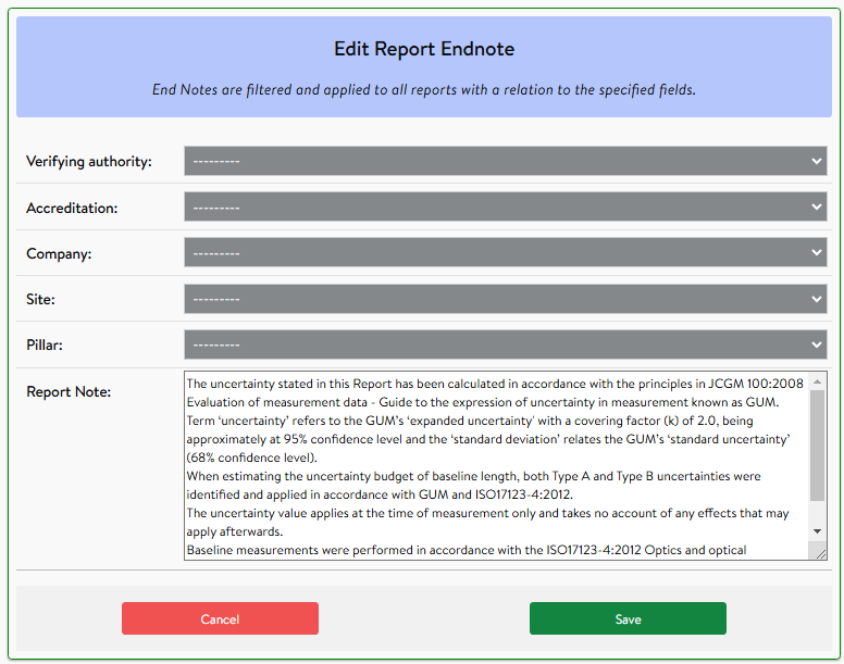
7.2.1 Verifying Authority Users
Verifying Authority users are able to apply additional endnotes with a greater range of filters. Leaving all of these fields blank will apply the endnote to either all of the EDMI or Baseline calibration reports.
Verifying authority: The note will be applied to all reports associated with baselines calibrated by the specified verifying authority.
Accreditation: The note will be applied to all reports associated with a specific accreditation issued to the verifying authority.
Company: The note will only be applied to reports for the specified company.
Site: The note will only be applied to reports associated with the specified calibration site.
Pillar: The note will only be applied to reports that use specified calibration pillar.
7.3 Interlaboratory comparison - Baselines
To assess the baseline calibration outcome in accordance with ISO 17025:2017, it is imperative to conduct an interlaboratory comparison. Therefore, the calibrated EDM baseline needs to be compared onto other EDM baseline/s (reference laboratory) to assess if it deliver the same results. The results can be assessed using the En value ('Error normalised'):
Where:
xlab = corrected distance of the calibrated baseline
xref = corrected distance of the reference baseline
Ulab = uncertainty of the distance at the calibrated baseline
Uref = uncertainty of the distance at the reference baseline
If the |En| ≤ 1 the results are satisfactory meaning the calibrated baseline (laboratory) is comparable to the reference baseline (laboratory) in terms of its performance. If the |En| > 1 the results are unsatisfactory (baselines are not providing the same results).
Copyright © 2020-2025 Western Australian Land Information Authority
Last updated: 24 November 2025
Please login or signup to manage and calibrate your staff.
Staff Calibration Technical User Manual
- 1. Introduction
- 2. About the Boya Staff Calibration Range
- 3. Staff Range Calibration
- 4. Barcode Staff Calibration
- 5. Conclusion
1. Introduction
Digital levelling systems have long been used by the Surveying and Engineering industry to determine height differences between any two or multiple locations for various applications. While the digital levelling instruments are incredibly accurate for their intended use, quick temperature changes, shock or stress, and wear and tear from daily usage can use signifant deviations and reduce the accuracy of the instrument over time. It is therefore, recommended to check and adjust the levelling instruments as per manufacturers specifications as well as their corresponding readings through established calibration procedures.
In Western Australia, Landgate is responsible for the national standard of measure for length, in this case, defined by the height difference or length measured in the vertical plane. In an effort to provide an accurate and a uniform system of levelling across the State, Landgate established a Staff Calibration Range at Boya in 2002. The range comprises 2 observing pillars and 21 pins set in a granite outcrop. The pins have been placed at optimum distances from the pillars and cater for testing over a 4 metre height difference. The relative height differences between the pins have been accurately determined by repeat observations using precision levels in conjunction with calibrated invar staves. Landgate regularly monitor and re-measure the Range to ensure its ongoing accuracy. Medjil provides an open-access platform to manage the digital levelling instruments and most importantly calibrate the ditital levelling staves using dedicated a dedicated calibration facility such as the Boya Staff Calibration Range.
This manual describes the steps and mathematical models used for:
- estimating the calibrated height differences and its uncertainty called as Staff Range Calibration
- computing the scale factor for a barcoded staff known as the Barcode Staff Calibration
2. About the Boya Staff Calibration Range
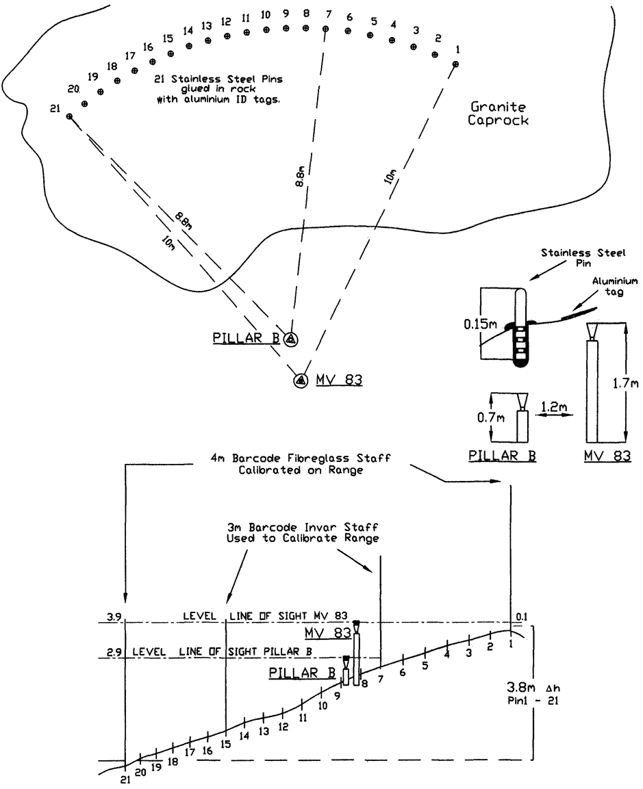
The Landgate barcode staff calibration range is located at the Land Surveyors Licensing Board's examination site at Boya and consists of 2 observing pillars and a series of 21 stainless steel pins set in a solid granite outcrop in a semi-arc rounding the two observing pillars.
The two observing pillars were first constructed beside a large piece of sloping granite which had the required 4 metres of height difference between top and bottom. The highest pillar is set at a comfortable observing height and the lowest a metre lower and closer to the rock and range.
The pins were glued into drilled holes in the granite while the observing pillars were concreted deep into the ground to ensure their stability. With the 3 metre invar staff, it was possible to observe from Pin 1 to 15 from the high pillar and from Pin 7 to Pin 21 from the lower pillar
Digital level set on Pillar MV 83 (high pillar)
The low pillar or Pillar B can be seen just below the high pillar..
Invar staff set on Pin 2
Invar staves set up on the pins are levelled and is held firmly by a bipole to main stability during the course of reading.
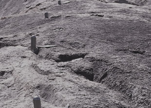
Stainless steel pins glued in granite rock
The pins were glued into drilled holes in the granite outcrop in an arc shape with a distance of about 10 metres from the high pillar and 8.8 metres from the low one.
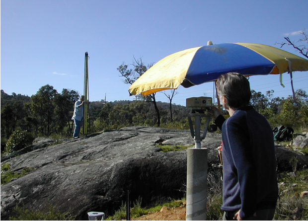
Observing from Pillar MV 83(high pillar).
With a 3 metre staff, readings can be done only for the first 15 pins using the high pillar.
3. Range calibration
The Landgate barcode staff calibration range is located at the Land Surveyors Licensing Board's examination site at Boya and consists of 2 observing pillars and a series of 21 stainless steel pins set in a solid granite outcrop.
3.1 Mathematical model for the calibration of the Barcode Calibration Range
For the the calibrations of the range the following mathematical model is used to fit the observations (height differences) between the pins. Redundant observations are required in order to carry out a least squares adjustment.
Where:
∆Hij = height difference between pins i and j
Mik = staff reading at pin i with a certified invar digital level
Mjk = staff reading at pin j with a certified invar digital level
k = observation set number. Each set contains several observations taken with the same instrument (level), staff and instrutment pillar
3.2 Observation equations and the least squares solution
The observation equations are derived from the mathematical model where the residual is the difference between the observed and the most probable height difference between the pins. One observation equation is formed for each observation. The initial most probabale height difference is adopted as the average height difference between the adjoining pillars if there are more than one observations.
Where:
vk = residual of the observation set between pins i and j in metres
For example, to determine the height interval $\Delta H$ between adjoining Pins i and j using 8 observations sets, the following equations can be used. $$v1 = \Delta H_{ij} - [M_{j1} - M_{i1}]$$ $$v1 = \Delta H_{ij} - [M_{j2} - M_{i2}]$$ $$v1 = \Delta H_{ij} - [M_{j3} - M_{i3}]$$ $$v1 = \Delta H_{ij} - [M_{j4} - M_{i4}]$$ $$v1 = \Delta H_{ij} - [M_{j5} - M_{i5}]$$ $$v1 = \Delta H_{ij} - [M_{j6} - M_{i6}]$$ $$v1 = \Delta H_{ij} - [M_{j6} - M_{i7}]$$ $$v1 = \Delta H_{ij} - [M_{j8} - M_{i8}]$$
Eq. 3.2 can be expressed in a matrix form:
Where:
$$A = \begin{bmatrix} 1 \\ 1 \\ 1 \\ 1 \\ 1 \\ 1 \\ 1 \\ 1 \end{bmatrix} X = \begin{bmatrix} \Delta H_{ij} \end{bmatrix} w = \begin{bmatrix} M_{j1} - M_{i1} \\ M_{j2} - M_{i2} \\ M_{j3} - M_{i3} \\ M_{j4} - M_{i4} \\ M_{j5} - M_{i5} \\ M_{j6} - M_{i6} \\ M_{j7} - M_{i7} \\ M_{j8} - M_{i8} \end{bmatrix} $$
A least squares adjustment computes the most probable values for the height differences between the pins. Any changes to the observations should be as small as possible. A least squares adjustment minimises the sum of the squares of the weighted residuals. The observation matrix (Eq. 3.3) can be combined with a weight matrix, $P$ (Eq. 3.5) to derive the best estimate for $\Delta H_{ij}$, represented by $x$ in Eq. 3.3 as follows:
$$x = (A^{T}PA)^{-1} A^{T}Pw \ \ (Eq. 3.4) $$
where P is a diagonal weight matrix that can be constructed from the a-priori standard daviations ($\sigma$) of each observation sets between pins i and j. For example, for the 8 observation sets as described above, the $P$ matrix is:
$$P = \begin{bmatrix} 1/\sigma_1^2 \\ & 1/\sigma_2^2 \\ & & 1/\sigma_3^2 \\ & & & 1/\sigma_4^2 \\ & & & & 1/\sigma_5^2 \\ & & & & & 1/\sigma_6^2 \\ & & & & & & 1/\sigma_7^2 \\ & & & & & & & 1/\sigma_8^2 \end{bmatrix} or P = [ \frac{1}{σ_{k}^2}] \ \ (Eq. 3.4)$$Where:
Where:
$\sigma$Mi = standard deviation of the observations to pin i
$\sigma$Mj = standard deviation of the observations to pin j
$\sigma$Tij = standard deviation of the temperature correction between pin i and j
Digital levels can now output standard deviations based on the number of readings per observation set by the users.
The uncertainty of the calibrated height difference is the a posteriori standard deviation of the adjusted height difference is and can be expressed at 95% confidence level by mupliplying it by coverage factor k = 1.96:
3.3 Time dependant range
Regular measurements of the Boya calibration range carried out by Landgate over the years indicated seasonal variations of up to 1 mm, thereby mandating the development of the time-dependent range which are used for (time depandant) staff calibration.
The range was measured every month over a period of two years and the observations used to estimate the following (see figure below) time dependant values of the range height differences.

The calibration range is monitored on a regular basis to ensure the validity of the model. Each new recalibration results are compared to the existing (avarege) range results to detect any anomalies.
4. Barcode Staff Calibration
4.1 Mathematical model for the computation of the correction factor of a barcode staff (the staff calibibration)
To estimate the the correction factor Cf of a barcoded staff the following mathematical model is used
Where:
∆Hij = certified range (or height difference between pins i and j)
Mi = barcoded staff reading at pin i
Mj = barcoded staff reading at pin j
4.2 Observation equations and least squares solution
Where:
Vij = residual of the correction factor of the height difference between pins i and j
For n pins the following set of equtions can be formed:
Where:
n = number of pins in the range.
The above equation can be expressed in a matrix notation:
Where:
$$A = \begin{bmatrix} 1 \\ 1 \\ .. \\ .. \\ 1 \end{bmatrix} X = \begin{bmatrix} C_{f} \end{bmatrix} w = \begin{bmatrix} \Delta H_{1,2}/[M_{2} - M_{1}] \\ \Delta H_{1,3}/[M_{3} - M_{1}] \\ .. \\ .. \\ \Delta H_{1,n}/[M_{n} - M_{1}] \end{bmatrix} $$
To determine the best estimate of $C_f$, the observation matrix (Eq. 4.4) can be combined with a weight matrix, $P$ (Eq. 4.6) as follows:
$$x = (A^{T}PA)^{-1} A^{T}Pw \ \ (Eq. 4.5) $$
where P is a diagonal weight matrix that can be constructed from a-priori standard daviations of each observation between pins 1 and $i$.
Where:
Where:
$\sigma$M1 = standard deviation of the observations to pin 1
$\sigma$Mi = standard deviation of the observations to pin i
$\sigma$T1i = standard deviation of the temperature correction between pin 1 and i
The standard deviations $\sigma_{M1}$ and $\sigma_{Mi}$ can be obtained from the staff readings. The uncertainty of the estimated correction factor is the a posteriori standard deviation calculated at 95% confidence level by multiplying with the coverage factor $k$ = 1.96.
$$\sigma_C = \sqrt(A^{T}PA)^{-1} \ \ (Eq. 4.8) $$4.3 Reducing the Correction Factor to a standart temperature
The staff correction factor $C_f$ is estimated at the average temparature during the staff calibration procedure without taking into account any previous calibrations. This is further reduced to a standard temperature T0, usually expressed at 25$^\circ$C using the following formula:
Where:
$C_f$ = the estimated staff correction factor with no tempeature correction
$T_{0}$ = standard temperature of 25.0$^\circ$C
$T_{obs}$ = average temperature [in $^\circ$C] during the staff calibration procedure
$\alpha$ = the coefficient of expansion of the barcoded staff
$C_{f_{T_{0}}}$ = the staff correction factor to be determined at 25.0$^\circ$C
4.4 Applying the Correction Factor $C_f$ to observed height differences
To correct the height differences obtained from the barcoded staff calibrated as above, the following formula is provided in the staff calibration certificate/report:
Where:
$\Delta H_C$ = corrected height difference
$T_{obs}$ = average temperature [in $^\circ$C]
$T_0$ = standard temperature of 25.0$^\circ$C
$\alpha$ = the coefficient of expansion of the barcoded staff
$C_{f_{T_{0}}}$ = the staff correction factor at T0
$\Delta H_{obs}$ = observed height difference
5. Conclusion
The Boya Staff Calibration Range and software developed by the then Department of Land Information (DLI) has enabled surveyors who use digital levels and barcode staves to calibrate their staves in a simple and cost effective manner for use in geodetic and other high order levelling. Both the calibration of the Range and Staves are based on the methods of least squares estimation, which is considered mathematically more rigorous. Medjil will update the estimated (monthly) average of the Staff Calibration Range whenever a new range measurement is added by Landgate. These (monthly) Range values are then used as a reference to calibrate other staves.
Copyright © 2020-2025 Western Australian Land Information Authority
Last updated: 24 May 2024